AI-Assisted Synthetic Time Series: Why Parametrized, Not Code Generation

If you're generating synthetic sensor data, you face a choice: write mathematical configurations manually (i.e. complex algorithm), or let an AI generate code to iterate and audit. 🐦‍🔥 PHOENIX offers a third path. Describe your signal in natural language, and an LLM-powered agent translates it into a validated JSON schema (e.g. frequency, amplitude, correlations, degradation parameters) that feeds a deterministic Python engine. Domain experts get an AI assistant that speaks their language. Developers get a practical pattern for building tools where LLMs parameterize instead of program, eliminating the security and reproducibility issues of code generation.

Design Philosophy

The AI layer in 🐦‍🔥 PHOENIX follows a parameterized generation architecture. The LLM does not generate Python code that gets executed. Instead, it translates natural language descriptions into a structured JSON parameter schema, which is then fed into a deterministic Python engine (TimeSeriesGenerator) that produces the data using NumPy and Pandas.

This separation has three key benefits:

Safety: No arbitrary code execution. The attack surface is limited to validated numeric parameters.
Determinism: The same parameters always produce the same class of output.
Auditability: Every generated time series can be fully described by its parameter set, which is stored alongside the data.

Architecture

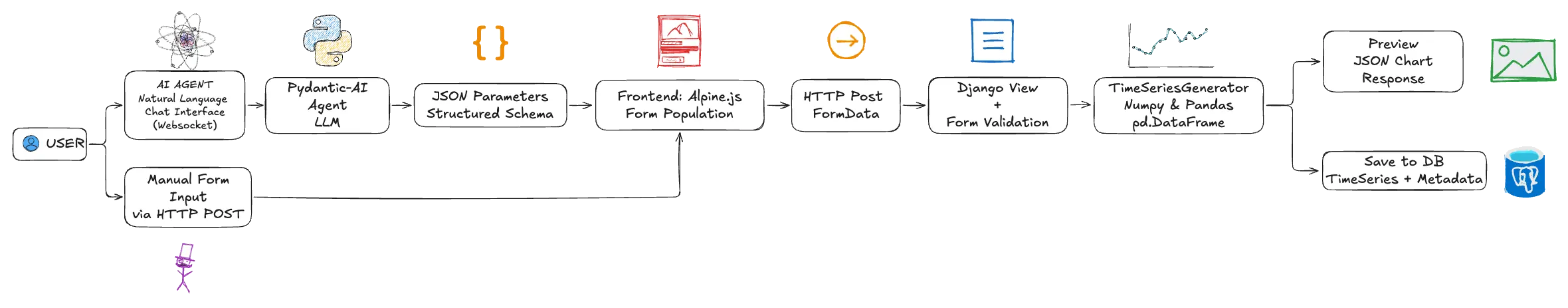
PHOENIX's generation pipeline consists of five main layers: user input (natural language or form) flows to a pydantic-ai LLM agent that produces structured JSON parameters, which then pass through Django form validation, into the TimeSeriesGenerator engine, and finally emerge as a stored DataFrame with full metadata. The architecture displayed below shows these layers and additional intermediate components.

AI Agent

The agent is responsible for interpreting natural language and producing structured time series generation parameters. It is composed of four primary code blocks:

Prompt schema: This is the time series domain knowledge. Basically, where we describe and teach the agent how to use the mathematical tools available in the project (e.g. noise generator) and how to interpret the user requests.
Pydantic-AI Factory: A module that converts LLM-style messages to pydantic-ai model messages.
User Context: Module for injecting user context. This is not widely used yet but has a potential to massively improve the TS synthetic generation experience based on the user profile. I expect that a mechanical engineer and a medical doctor will express themselves differently to the agent. Teaching the agent how to interpret the language used by the user based on their background will (I believe) prove to be a powerful concept.
Handlers: Event stream handler for logging and monitoring.

The time series generation agent has no tools, no database access, and no file system access. It can only produce text. The conversation history is managed server-side and is scoped to the user session.

Chat

The chat interface handles real-time communication (WebSocket) between the browser and the AI agent. Beyond text input, the chat interface supports image uploads and speech-to-text recognition, both of which significantly improve the user experience for time series generation.

Users can photograph or screenshot an existing signal plot and send it directly to the agent, which interprets visual characteristics (e.g. shape, frequency content, amplitude, noise levels, trends) and produces matching generation parameters.

These multimodal inputs feed into the same AI pipeline: the LLM interprets the content and responds with the standard JSON parameter block, keeping the architecture and validation layers unchanged.

Python Generation Engine

This is the deterministic core of 🐦‍🔥 PHOENIX. It receives validated parameters and produces synthetic time series data using pure Python numerical computation. The engine is built around the TimeSeriesGenerator class, which exposes an API for constructing signals as a superposition of a baseline mean, linear trends, sinusoidal oscillations, Gaussian noise, and more. For multi-channel scenarios, cross-channel correlations are applied via Cholesky decomposition on the correlation matrix.

All heavy computation is delegated to NumPy vectorized operations, and the output is returned as a Pandas DataFrame with a DatetimeIndex. Because the engine operates exclusively on bounded, validated numeric inputs (never on generated code) it is both fast (sub-second a 10,000 data points TS) and inherently safe.

Time Series Generator

At the core of the application is the TimeSeriesGenerator class is a deterministic Python Engine. It is a pure Python engine built on NumPy and Pandas that transforms validated parameters into time series data using a “Method Chaining API”, as shown in the code below:

ts = (TimeSeriesGenerator()
      .with_duration(days=7, time_step_seconds=60)
      .with_base_signal(mean=100, noise_amplitude=5.0)
      .with_trend(slope=0.5)
      .with_oscillation(frequency_hz=0.001, amplitude=10.0)
      .generate())

The generated signal is a superposition of independent components. For example,

where each component is computed as a NumPy array operation. Furthermore, each component of the signal is configured and modelled as a Pydantic BaseModel with validation.

The generator returns a Pandas DataFrame with a DatetimeIndex:

Single-channel: One column named value
Multi-channel: One column per channel, named after the channel

This DataFrame is then serialized into Plotly.js trace format for preview, or stored as JSON in the database for persistence.

Data Storage

Saved time series are stored in the database and linked to the user account. Each series contains two key pieces: the actual data (timestamps and channel values) and the complete generation recipe (parameters). This "recipe" approach means you can regenerate identical data anytime, or create variations by changing a single parameter.

🐦‍🔥 PHOENIX stores generated data (less that 10,000 data points) in a format optimized for the quick previews and interactive charts you see in the interface. For larger time series or data uploaded from external sources, the system automatically uses a different storage approach designed for time series at scale.

Frontend

The 🐦‍🔥 PHOENIX interface is built with Django templates and styled with modern CSS frameworks, with Alpine.js handling the interactive behavior you see when adding channels, configuring oscillations, or editing correlations.

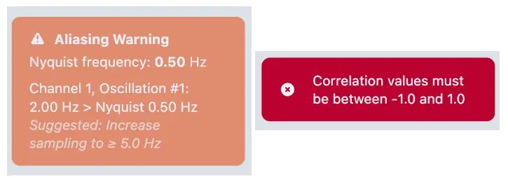
Client-side validation catches issues like aliasing problems before you even preview, but the real validation happens server-side in Python through Django forms and Pydantic models.

When you click "Preview," your parameters go to a Python view that instantiates the TimeSeriesGenerator, runs the NumPy operations, and serializes the DataFrame into Plotly.js chart format. The result: fully interactive charts where you can zoom into specific time ranges, toggle channels on and off, and hover for exact values.

The Prompt Engineering Layer

The system prompt is an ever growing structured document that gives the LLM everything it needs to produce valid generation parameters. It is divided into multiple sections and new sections are added as required or requested.

Schema Definition

The prompt defines the exact JSON schema the LLM must produce, including every field, its type, and valid ranges. The schema covers all the parameters available in the side bar navigation (e.g. Time Configuration, Channels, Correlations) and special sections to improve the agent’s domain knowledge and dexterity when using the available mathematical tools at its disposal. Examples of these are:

Nyquist-Shannon Compliance: The prompt contains explicit instructions for aliasing prevention. The LLM is instructed to verify every oscillation against the Nyquist limit before producing its JSON, and to either increase the sampling frequency or lower the oscillation frequency if a violation would occur.
Nonlinear Trend Approximation: Since the generator only supports linear trends natively, the prompt teaches the LLM a technique for approximating nonlinear curves using long-period oscillations (e.g. exponential growth, logarithmic saturation, s-curve).
Domain Knowledge: The prompt encodes typical defaults for industrial sensor types (vibration, temperature, pressure, flow, acoustic, electrical) so the LLM can make informed choices when users describe signals by domain rather than by mathematical properties.

Image Interpretation

The agent agent accepts chart images and can interpret visual characteristics (signal shape, frequency content, amplitude ranges, noise levels) to infer generation parameters. This is enabled by the multimodal capabilities of the underlying LLM.

Example: Global Warming Temperature Trend

What better that a aI did a nice test in which I asked the AI to simulate the global warming temperature trend, fed it an image and in a single try this was the result:

Speech Interpretation

Speech-to-text allows users to verbally describe complex multi-channel setups hands-free, which is particularly useful for engineers working in industrial environments where typing may be impractical. These multimodal inputs feed into the same AI pipeline: the LLM interprets the content and responds with the standard JSON parameter block, keeping the architecture and validation layers unchanged.

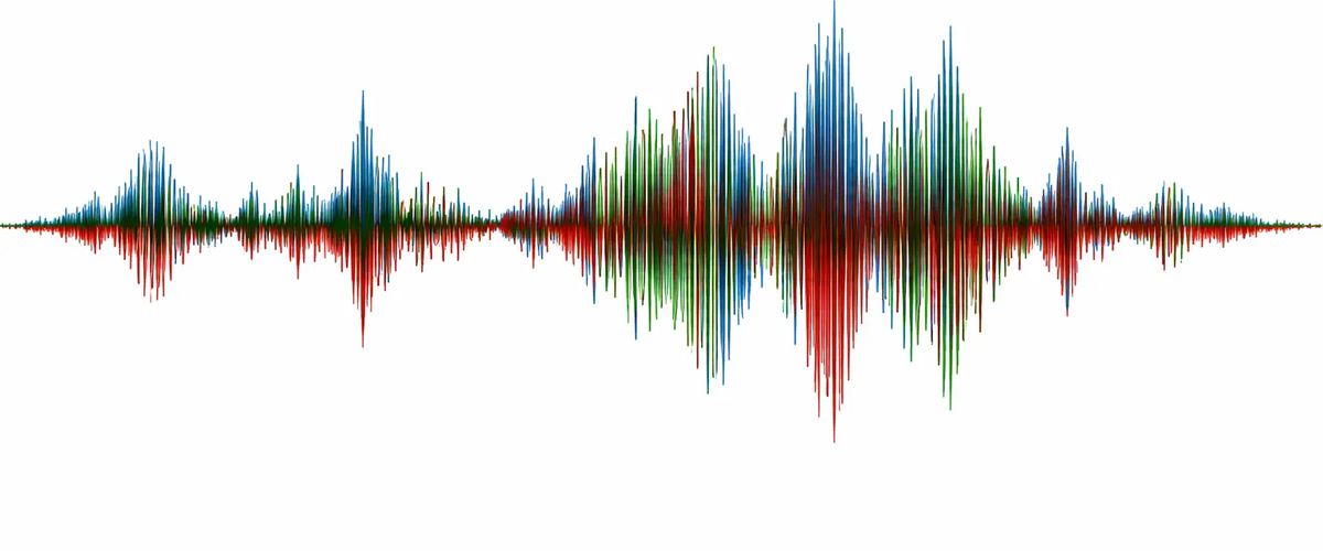
Example: Seismograph data

I wanted to test the agent capabilities to produce a time series from a screenshot of actual data or from a prompt given by a domain expert. For that, I used the seismograph image with S-wave and P-wave (Wikimedia)

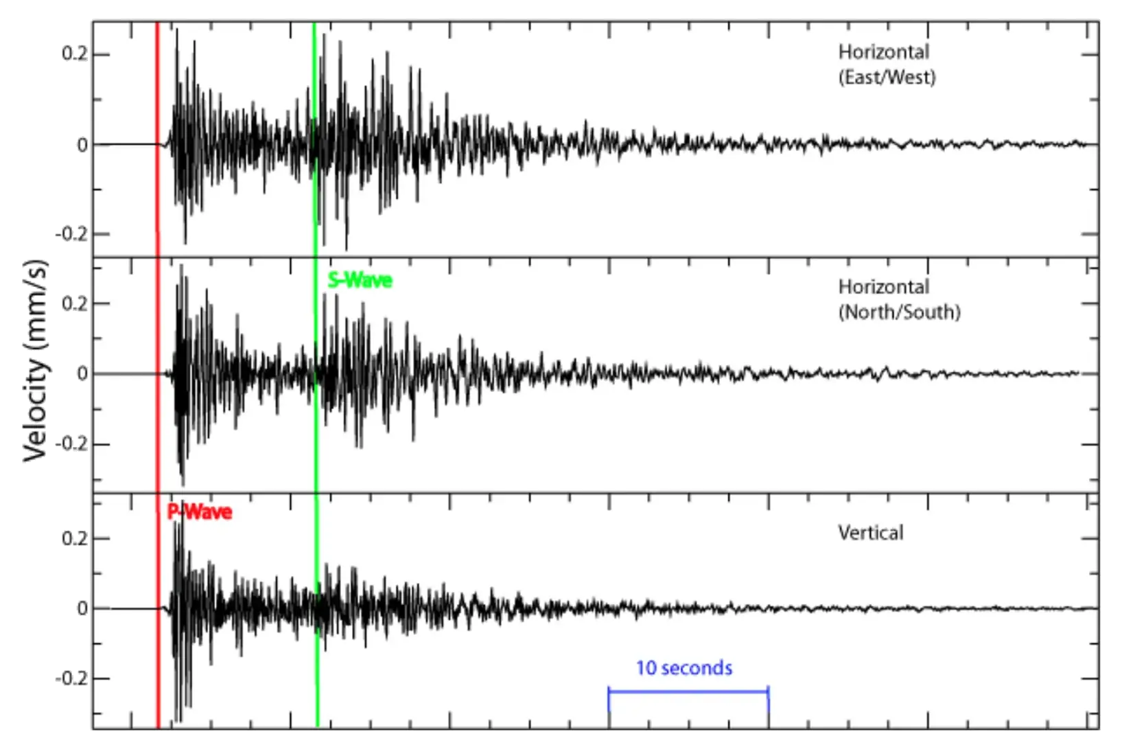
https://commons.wikimedia.org/wiki/File:Seismogram.gif

Giving the agent the image and the following prompt

Generate a 60-second seismograph recording similar to the one in the image for the Horizontal (East/West) event.

and some additional instructions (see video) after the first attempt, produces a nice simulation of the seismograph data.

Alternatively, if you know what you want and and can provide the agent with clear instructions from a domain point of view, it will do a very nice job straight away. This is a “domian-driven” prompt and the result:

Simulate a 60-second vertical seismograph recording with a P-wave arrival at 5 seconds and an S-wave arrival at 15 seconds. The P-wave should have moderate amplitude (~50 mm/s) with a frequency around 8 Hz and light damping. The S-wave should be larger (~120 mm/s) with a lower frequency around 3 Hz. Add ambient ground noise of about 0.5 mm/s. Use realistic seismic parameters for a local earthquake.

Why Parameterized Generation and Not Code Generation

An alternative architecture would be to force the LLM to generate Python code (e.g., NumPy scripts) that gets executed directly. 🐦‍🔥 PHOENIX deliberately avoids this for several reasons:

Security

No code execution and all numeric inputs are bounded. A code generation approach would require sandboxing, code review or deploying execution environments.

Validation

Full server-side validation of every parameter. Otherwise, the application would have to validate arbitrary code for correcteness and safety.

Reproducibility

This is a simple one. Parameters are store in the DB and identical re-generation is a one-click process. Code generation requires storing (who knows how many lines of) code and an engine to re-execute it on demand. Additionally, the dependencies management could become a problem as the code generation DB grows.

User Control

Users see and can modify every parameter in the form (UI). This creates low barriers for non-coders. Otherwise, users must understand generated code to modify it.

Error Handling

Validation errors map to specific form fields. Code execution generates runtime errors. This are in most cases opaque and not easy to understand for non-developers.

Flexibility Tradeoff

This TS generation is limited to the superposition model. With code it is possible to express any computable time series. The flexibility tradeoff is intentional. The superposition model (mean + trend + oscillations + noise) covers the vast majority of synthetic time series use cases in industrial settings. The nonlinear trend approximation technique (long-period oscillations) extends coverage to exponential, logarithmic, and sigmoid shapes without requiring arbitrary code. Furthermore, if a a user (or myself) come up with a request that can’t be satisfactory fulfilled by the AI Agent, the prompts can be improved or extended or new mathematical tools can be added to the toolbelt the ai-agent has access to.

Known Limitations

While the AI-powered time series generator excels at creating controlled synthetic data with well-defined mathematical characteristics, it has inherent limitations when replicating highly complex real-world signals. The generator models signals as combinations of fundamental mathematical components (e.g. periodic oscillations, linear trends, exponential decays, and random noise). Real-world sensor data, however, often exhibits phenomena that cannot be decomposed into these simple building blocks: time-varying spectral content, complex amplitude modulation from interference effects, chaotic dynamics, fractal patterns, and non-stationary stochastic behavior. The generator is best suited for creating idealized signals for algorithm development, educational demonstrations, and controlled testing scenarios where you need precise control over signal parameters and understand the ground truth. For applications requiring high-fidelity replicas of real sensor data, such as training production machine learning models or validating systems against authentic operational conditions, you should use actual recorded data or domain-specific physics-based simulation tools. Users can achieve more realistic complexity by layering multiple signal components with varying parameters, but this remains a mathematical approximation rather than a true physical simulation of the underlying data-generating process.