Multichannel Correlated Time Series

🐦‍🔥 PHOENIX has the ability to generate multichannel time series with statistical relationships (correlations or not) between channels. If you have a good understanding of correlated signals, feel free to skip the first part of the article and got to the step-by-step tutorial on how generate a multichannel correlated time series, or jump straight to the Kronts website to do it.

Why Generate Multichannel Time Series?

Multichannel generation allows you to create datasets with multiple independent or correlated signals sharing the same time axis. This is essential for simulating multi-sensor systems common in industrial environments.

What Are Multichannel Time Series?

Multichannel time series have:

• Single time axis: All channels share the same timestamps
• Multiple data columns: Each channel has its own values
• Independent or correlated: Channels can be statistically related

A single channel time series would look like this:

Timestamp Value

2024-01-01 00:00:00 100.5

2024-01-01 00:00:01 101.2

2024-01-01 00:00:02 99.8

While a multichannel time series (3 channels) would look like this:

Timestamp X-Axis Y-Axis Z-Axis

2024-01-01 00:00:00 0.5 0.3 -0.2

2024-01-01 00:00:01 0.6 0.4 -0.1

2024-01-01 00:00:02 0.4 0.2 -0.3

When to Use Multichannel Time Series

When should you use multichannel generation? When you have a problem involving multiple related sensors. In other words, what is your use case or problem to solve in which there are multiple time series and you suspect there is a correlation between them. There are many fields of engineering in which sensor data is correlated. The following are just two examples I was exposed to.

Vibration Monitoring

An example of correlated signals are forces on structures or components (e.g. naval hydrofoils) using accelerometers. This typically involves:

• 3 accelerometers (X, Y, Z axes)
• Partially correlated (mechanical coupling)
• Different vibration characteristics per axis

In these measurements, the three accelerometers don't move identically; each axis experiences different forcing. Understanding how X, Y, and Z axes couple tells us about structural failure modes, something you can't learn from studying them independently.

Synthetic time series with known correlations provide canonical data under controlled conditions to develop algorithms that detect frequency-resolved correlations between input and output signals and identify resonant behavior under realistic constraints.

Environmental Monitoring and Wave-Structure Interaction

Wave-structure interaction in coastal and ocean environments presents a rich domain for studying highly correlated data. Submerged coastal structures exemplify this challenge well. Understanding how waves interact with structures like breakwaters, seawalls, or offshore platforms requires monitoring highly correlated signals that reveal the coupling between fluid dynamics and structural response. A typical monitoring setup includes pressure sensors on the structure surface, accelerometers measuring structural vibration (typically in surge, sway, and heave directions), and water surface elevation sensors nearby. These channels are tightly correlated because they're all driven by the same incident wave field, but the correlation structure encodes critical information about energy transfer between the fluid and structure.

How to Generate Multichannel Correlated Time Series with PHOENIX in 6 Steps

We will generate a realistic synthetic sensor data set from an ideal gas experiment. An ideal gas system is simple enough to verify your setup, yet realistic enough to prepare you for messier real-world correlations where the underlying relationships are unknown.By the end, you will have created a two-channel time series representing temperature and pressure readings from a sealed container of gas, complete with correlated signals, and realistic noise patterns.

Background: The Ideal Gas Law

The ideal gas law states:

Where:

• P = Pressure (Pa)
• V = Volume (m³)
• n = Amount of substance (mol)
• R = Universal gas constant (8.314 J/(mol·K))
• T = Temperature (K)

For a sealed container (fixed V and n), pressure is directly proportional to temperature. This means that when temperature rises, pressure rises proportionally. This physical relationship makes an ideal gas system a perfect example for multi-channel generation: two measured quantities that are strongly correlated by a known physical law.

Step 1: Open PHOENIX

Navigate to 🐦‍🔥 PHOENIX from the main navigation. You will see the generation interface with a sidebar on the left for configuration and a blank chart area on the right.

Step 2: Configure the Time Axis

All channels share the same time axis, so we configure this first.

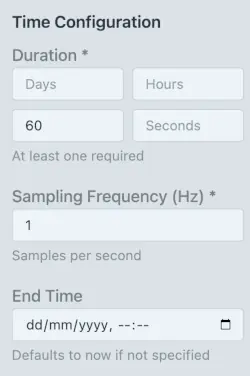
In the Time Configuration section of the sidebar, enter:

• Duration = 2 hours
• Sampling Frequency = 0.5 Hz

Leave the End Time empty, unless you want to have a specific end date for the time series.

Step 3: Create the Temperature Channel

By default, 🐦‍🔥 PHOENIX starts with a single channel. This will become our Temperature channel.

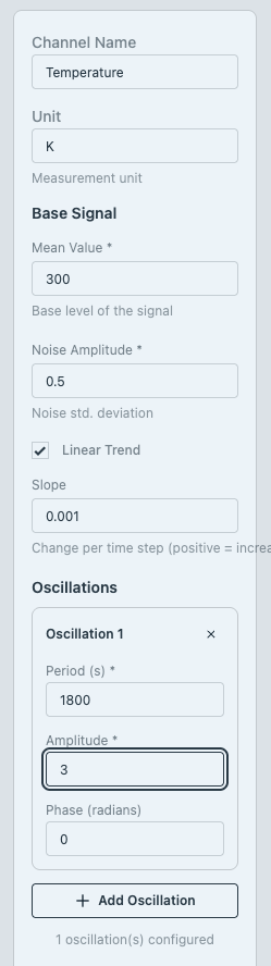
Click on the Channel 1 tab (it should already be active) and configure:

• Channel Name = Temperature
• Unit = K

Base Signal

• Mean = 300
• Noise Amplitude = 0.5

This simulates a baseline temperature of 300 K (27°) with a sensor noise of ±0.5 K, typical for an industrial thermocouple.

Linear Trend

Assume we are in closed rooms (e.g. laboratory) and it will gradually warm up during the data acquisition period. A realistic warm up rate would be 0.001 K per time step, a subtle but detectable rise. Enable the trend and set:

• Trend Slope = 0.001

Oscillations

In our hypotetical laboratory there is a ventilation system (HVAC) with a 30 min on/off cycle. This will generate a temperature swing of about ±3 K around the mean (a realistic HVAC-driven fluctuation).

Enable Oscillations and configure:

• Period (seconds) = 1800
• Amplitude = 3
• Phase = 0

This oscillation creates the dominant periodic pattern in the temperature signal.

Step 4: Create the Pressure Channel

Click the Add Channel button. A new tab labelled “Channel 2” appears. Click on it to make it active and fill in the Pressure parameters:

• Channel Name = Pressure
• Unit = kPa

Base Signal

For our sealed container, using assumed values for the ideal gas formula.

• Mean = 124
• Noise Amplitude = 0.8

This produces an equilibrium pressure at 300 K with a transducer noise of ±0.8 kPa, realistic for an industrial sensor.

Linear Trend

Enable the trend:

• Trend Slope = 0.0004

Pressure rises proportionally to temperature. Since the temperature trend is 0.001 K/step and the sensitivity is roughly 0.415 kPa/K (from nR/V), the pressure trend is ~0.0004 kPa/step.

Oscillations

Click Add Oscillation and enter the following parameters:

• Period (seconds) = 1800
• Amplitude = 1.25
• Phase = 0

These parameters simulate a pressure with the same 30 min cycle as the temperature sensor (pressure follow temperature as per the gas law). Since the temperature amplitude is 3 K. Pressure sensitivity (nR/V) ≈ 0.415 kPa/K, so pressure amplitude ≈ 3 × 0.415 ≈ 1.25 kPa.

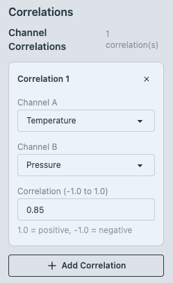
Step 5: Add Channel Correlation

Temperature and pressure in an ideal gas are strongly positively correlated. We need to tell 🐦‍🔥 PHOENIX about this physical relationship.

Scroll down to the Channel Correlations section (this appears automatically when you have 2 or more channels).

1. Click Add Correlation
2. Set Channel A to Temperature
3. Set Channel B to Pressure
4. Set Correlation to 0.85

Why 0.85 and not 1.0? In a perfect ideal gas with perfect sensors, the correlation would be 1.0. We use 0.85 to account for:

• Independent sensor noise on each measurement
• Small deviations from ideal gas behaviour
• Measurement timing differences

This creates a realistic scenario where the signals are strongly related but not identical. In practice, you'll rarely know the true correlation. You'll estimate it from data or domain knowledge. This exercise teaches you to think about what correlation value makes sense for your problem.

Step 6: Preview the Data

Click the Preview button at the bottom of the sidebar. 🐦‍🔥 PHOENIX will generate the two-channel time series and displays an interactive chart. You should see:

As defined in the parameters, you will get two coloured traces, one for Temperature, one for Pressure, with a shared time axis. The two time series are correlated, have the the same 30 min oscillation clearly visible in both signals, with a subtle upward trend over the full 2-hour window and random noise, adding realistic jitter to both signals.

What to Look For

• Correlation: Click on the Temperature legend entry to hide it. Observe the Pressure trace alone. Then toggle it back and hide Pressure. Both should show the same general wave pattern.
• Scale difference: Temperature oscillates around 300 K while Pressure oscillates around 124.7 kPa. Different scales, but the patterns are synchronised.
• Noise difference: Pressure (noise=0.8) should look slightly noisier relative to its oscillation amplitude than Temperature (noise=0.5).
• Trend: Look at the starting values versus the ending values. Both channels should end slightly higher than they started.

Once you preview, you can Export or Iterate. Most users iterate 2–3 times, adjusting noise or correlation before settling on a dataset.

Concluding Remarks

For me this is very exciting. 🐦‍🔥 PHOENIX multichannel generation lets you create physically realistic datasets where signals share a common time axis and can be correlated. Allowing us to model physical relationships between measured quantities, in this case, the ideal gas law linking temperature and pressure. Additionally, you can simulate independent data degradation (read more here) per channel to create realistic data quality scenarios where different sensors fail in different ways. This foundation opens the door to simulating complex multi-sensor scenarios where individual channel degradation modes interact unpredictably. Try it yourself.

Exercises

After you completed the Ideal Gas synthetic time series generation presented above, try the following variations to deepen your understanding.

Exercise 1: Add a Third Channel for Volume

In reality, containers can expand slightly under pressure. Add a third channel for Volume:

• Mean: 0.01 m³
• Very small noise (0.0001)
• Weak negative correlation with Pressure (-0.1)
• No oscillation (rigid container)

Exercise 2: Simulate a Cooling Event

Change the Temperature trend slope to a negative value (-0.002) to simulate the lab cooling down. Observe how the Pressure channel follows.

Exercise 3: Phase Lag

In some systems, pressure responds to temperature with a delay. Set the Pressure oscillation phase to 0.3 radians (≈ 17 seconds delay) and observe the subtle timing offset in the preview.

Exercise 4: Increase Correlation

Set the correlation to 0.95 and regenerate. Compare how closely the channels track each other versus the 0.85 configuration.