PHOENIX: Synthetic Time Series Generator App | Kronts

Data scientists frequently encounter a recurring challenge: needing test data for development work without access to production datasets. The typical pattern unfolds the same way—identifying a processing task, knowing the approach but lacking data, and writing throwaway scripts to generate test sets that end up lost or buried deep in obscure repositories.

To address this, we built 🐦‍🔥 PHOENIX, the first application in the Kronts ecosystem for systematising synthetic data generation.

PHOENIX: Synthetic Time Series Generator

This is a tool that enables users to create realistic, configurable time series data for testing, training, and simulation purposes. It provides an interactive interface where users can define time configurations, base signals, oscillations, and data degradation patterns to generate custom time series datasets. Key capabilities include:

Configurable Time Parameters: Define start/end times, sampling rates, and temporal characteristics
Base Signal Configuration: Set up foundational signal patterns and behaviors
Oscillation Controls: Add periodic variations and cyclical patterns to the data
Transient Controls: Include response from an equilibrium or a steady state
Data Degradation Settings: Simulate real-world data quality issues like noise, gaps, or drift
Interactive Preview: Generate and visualize time series in real-time before saving
Multiple Export Formats: Download generated data as CSV, Excel (.xls), or JSON
Save & Regenerate: Save time series configurations with names and descriptions for future reuse
Responsive Chart Display: Interactive Plotly.js-powered visualization with zoom and exploration capabilities

Basic Signal Generation

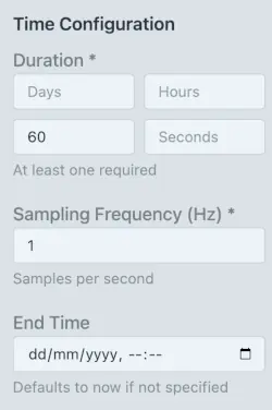
The basis of the signal generation is simple. First, input the time parameters in the Time Configuration section. Basically, define the duration of the signal and the sampling frequency. If there is a need to control the time stamp of the signal, enter the end time of the signal (i.e. the time stamp of the last data point). There are default parameters in place to generate a simple signal and iterate from it.

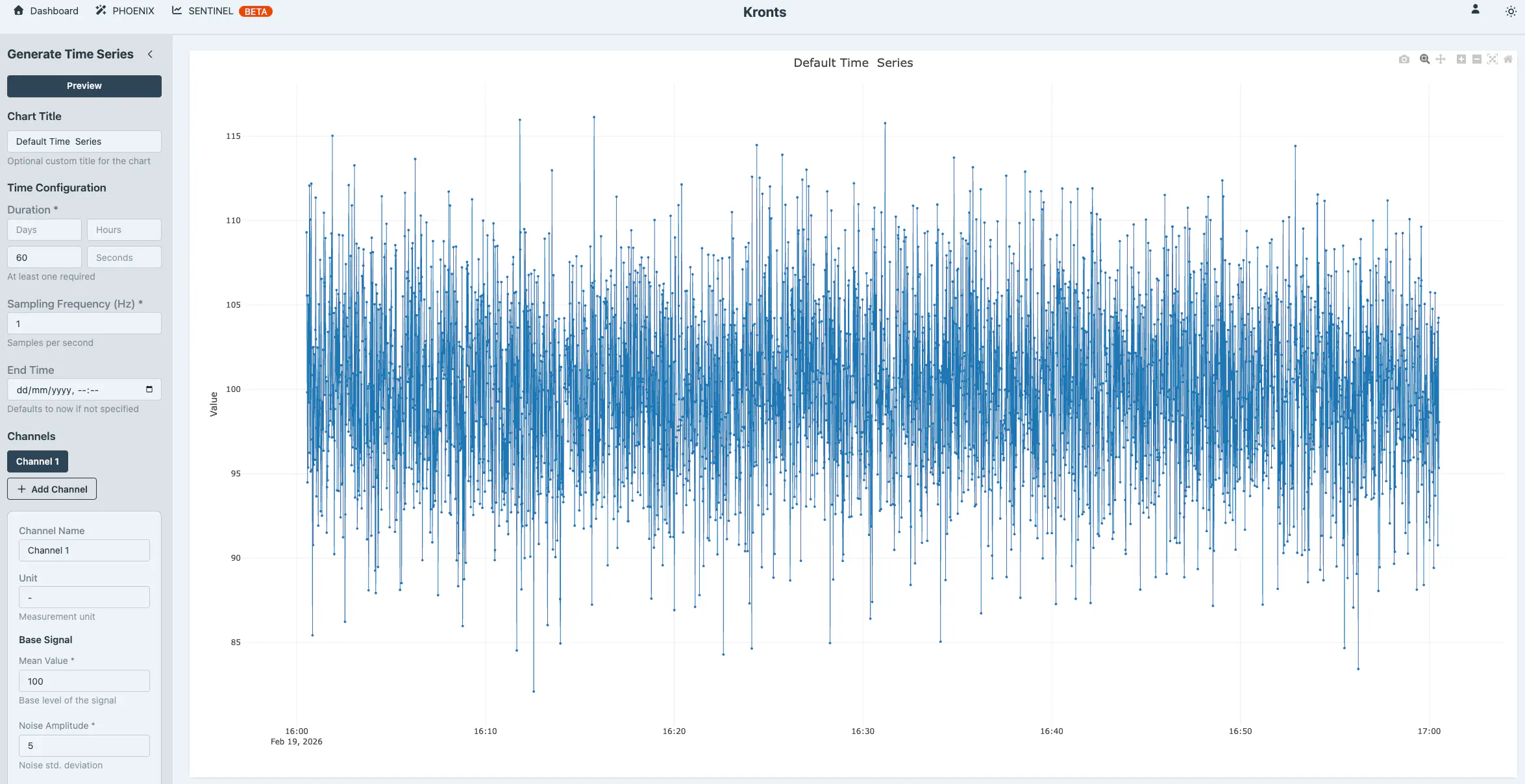
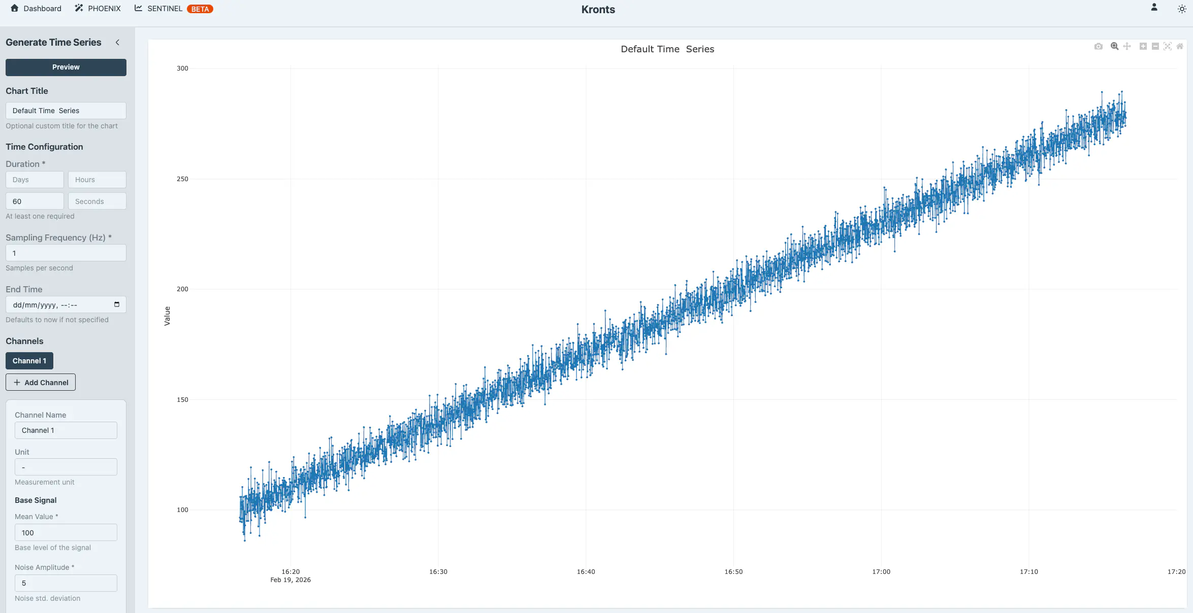
To add more features to the base signal, you can control three elements that shape its overall character: the mean value, which shifts the signal up or down along the vertical axis; random noise, which introduces realistic variability around the signal's core pattern; and a linear trend, which applies a gradual upward or downward drift over time. With the default values already in the UI we get a flat time series with noise.

And adding a linear trend with a slope of 0.05 transforms it to the following.

Very simple and fast. Now the user can chose to iterate, download the data as CSV, XLS or JSON format or save it to their personal space.

Generating Complex Time Series

PHOENIX offers capabilities to generate increasingly complex signals, with seasonal components (e.g. weather patters, physical phenomena) and poor quality (e.g. missing data, outliers). The primary mathematical tool used by the Time Series Generator are oscillations.

Oscillations

In digital signal processing (DSP), it is well established that any signal can be decomposed into a, potentially infinite, sum of sinusoids, each with its own frequency, amplitude, and phase. Mathematically:

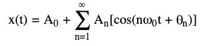
Without diving too deep into formal definitions, this means we can mix and match different wave patterns to build realistic, complex signals. This is a powerful and versatile concept applied to time series generation that can be applied to countless engineering problems. By superimposing multiple waves, we can generate signals that represent or simulate a wide range of complex physical phenomena.

Rather than spending time on manual research or calculations to determine the right parameters, this is a task that can be delegated to an AI. We prompted Claude to suggest parameters for PHOENIX to simulate physical phenomena requiring multiple oscillations. We got multiple suggestions, below are two examples. We also asked Claude to provide the parameters in a JSON format following the PHOENIX available controls.

Rotating Machinery with Harmonics

This Simulates a motor or pump with a fundamental frequency and harmonic vibrations:

Primary oscillation: 10 Hz (0.1s period) - main rotation frequency
2nd harmonic: 20 Hz - bearing defect
3rd harmonic: 30 Hz - gear mesh frequency

{
  "duration_minutes": 1,
  "frequency": 200,
  "mean": 50,
  "noise_amplitude": 2,
  "trend_slope": 0.001,
  "oscillations": [
      {"period_seconds": 0.1, "amplitude": 10, "phase": 0},
      {"period_seconds": 0.05, "amplitude": 3, "phase": 0.5},
      {"period_seconds": 0.033, "amplitude": 1.5, "phase": 1.2}
  ]
}

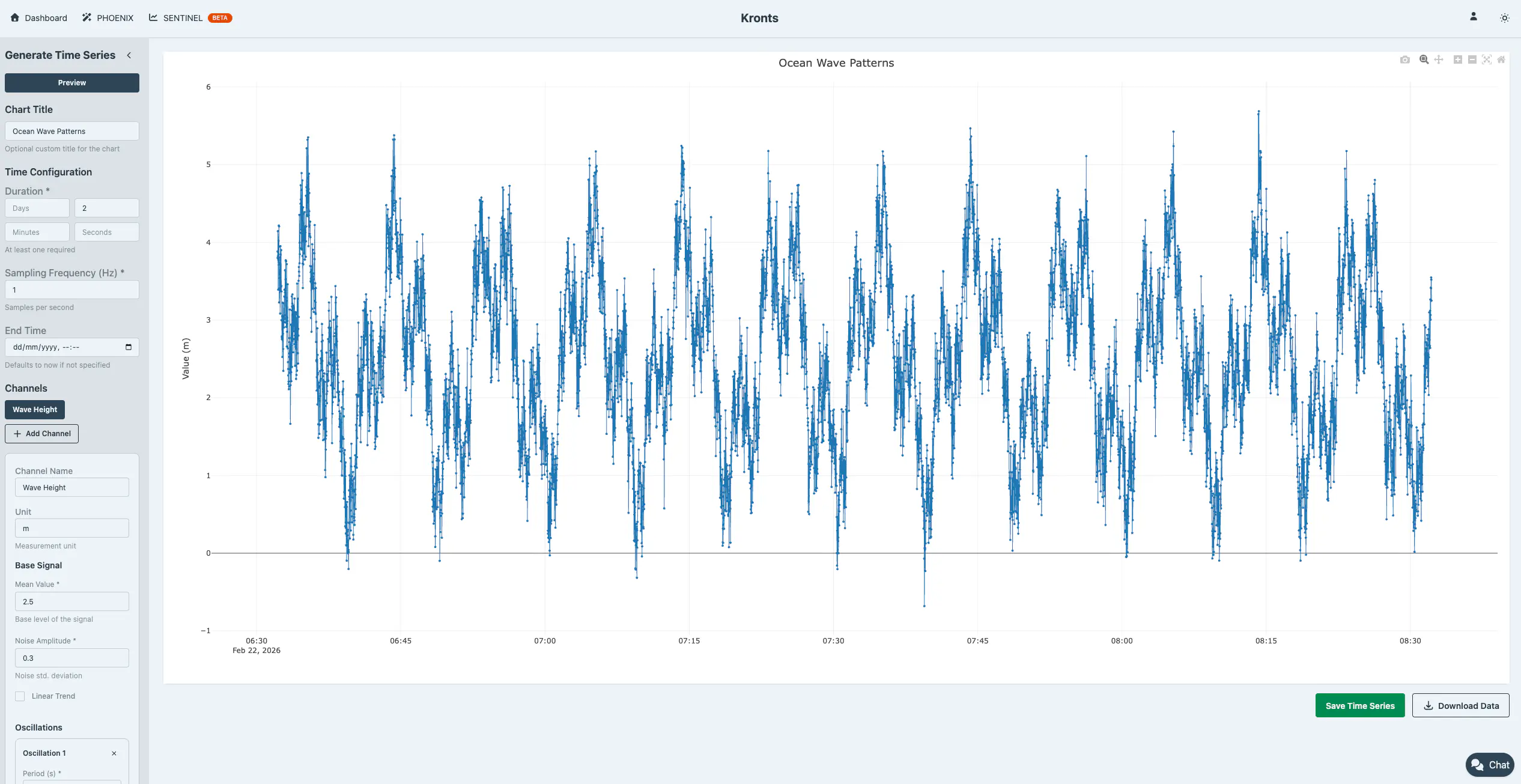
Ocean Wave Patterns

Simulates multiple wave frequencies (swell + wind waves):

Long period swell: 10 minutes
Medium waves: 3 minutes
Short period wind waves: 45 seconds

{
  "duration_hours": 2,
  "frequency": 1,
  "mean": 2.5,
  "noise_amplitude": 0.3,
  "oscillations": [
     {"period_seconds": 600, "amplitude": 1.2, "phase": 0},
     {"period_seconds": 180, "amplitude": 0.8, "phase": 1.57},
     {"period_seconds": 45, "amplitude": 0.4, "phase": 0.5}
  ]
}

Degraded Data Quality Simulation … and something more

Real-world data is messy. Sensors fail, transmissions drop packets, and measurements spike unexpectedly. PHOENIX lets you inject these realistic imperfections into your synthetic data so you can test how your processing workflows handle the chaos.

Remove data points randomly (by count or percentage) to simulate sensor dropouts or transmission gaps.

Insert outliers using constant values, random ranges, or multiplication factors to replicate measurement anomalies and edge cases.

By testing against degraded data now, you catch problems before they hit production.

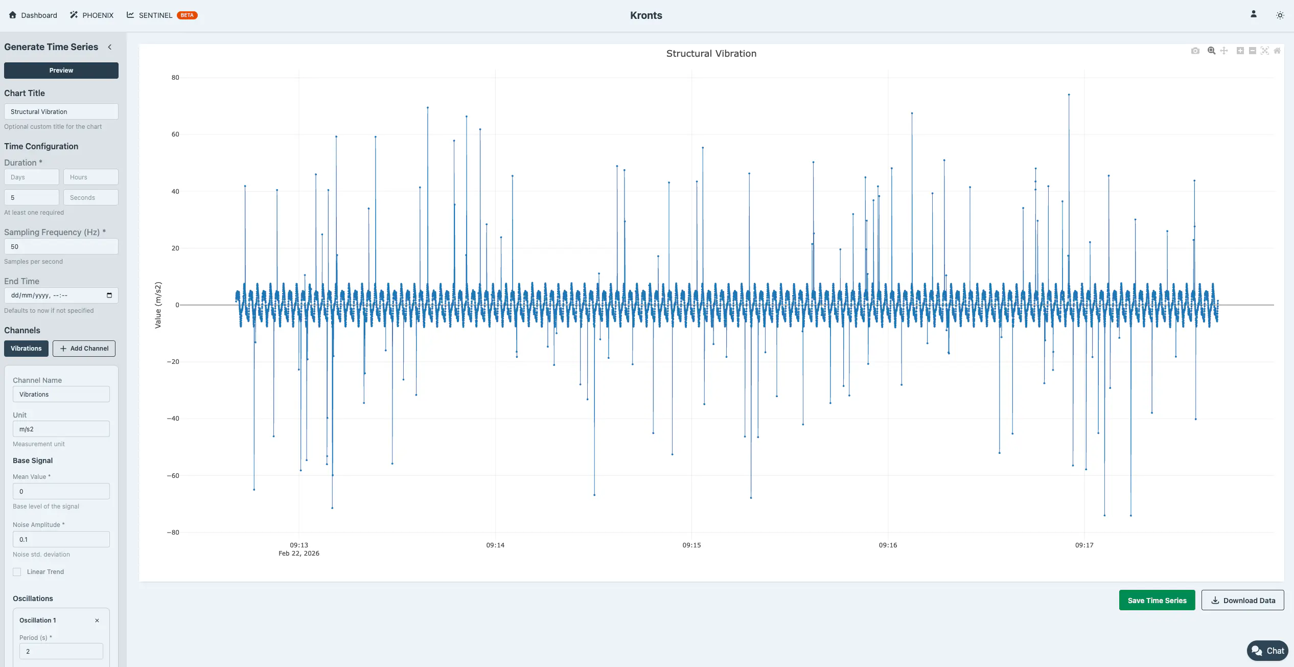
Interesting Example

As mentioned before, Claude used these features to simulate another interesting time series. Instead of using the outlier generation as actual outliers, Claude used it as a feature of the signal, outliers as shock events in an earthquake.

3. Seismic/Structural Vibration

Simulates building response to multiple modal frequencies:

1st mode: 0.5 Hz (2s period) - fundamental frequency
2nd mode: 1.25 Hz - second structural mode
3rd mode: 2.5 Hz - higher mode
Includes shock events (outliers)

{
  "duration_minutes": 5,
  "frequency": 50,
  "mean": 0,
  "noise_amplitude": 0.1,
  "oscillations": [
      {"period_seconds": 2, "amplitude": 5, "phase": 0},
      {"period_seconds": 0.8, "amplitude": 2, "phase": 0.3},
     {"period_seconds": 0.4, "amplitude": 1, "phase": 0.9}
  ],
  "outlier_mode": "percentage",
  "outlier_percentage": 1,
  "outlier_value_mode": "factor",
  "outlier_factor": 10
}

Structural vibrations synthetic time series

Interactive Development

Don’t commit to storage blindly. Preview your generated time series in real-time, adjust parameters on the fly, and instantly see how changes affect your signal. Iterate until the output matches your requirements, then save to your library. This tight feedback loop means you spend less time tweaking configurations and more time validating your algorithms.

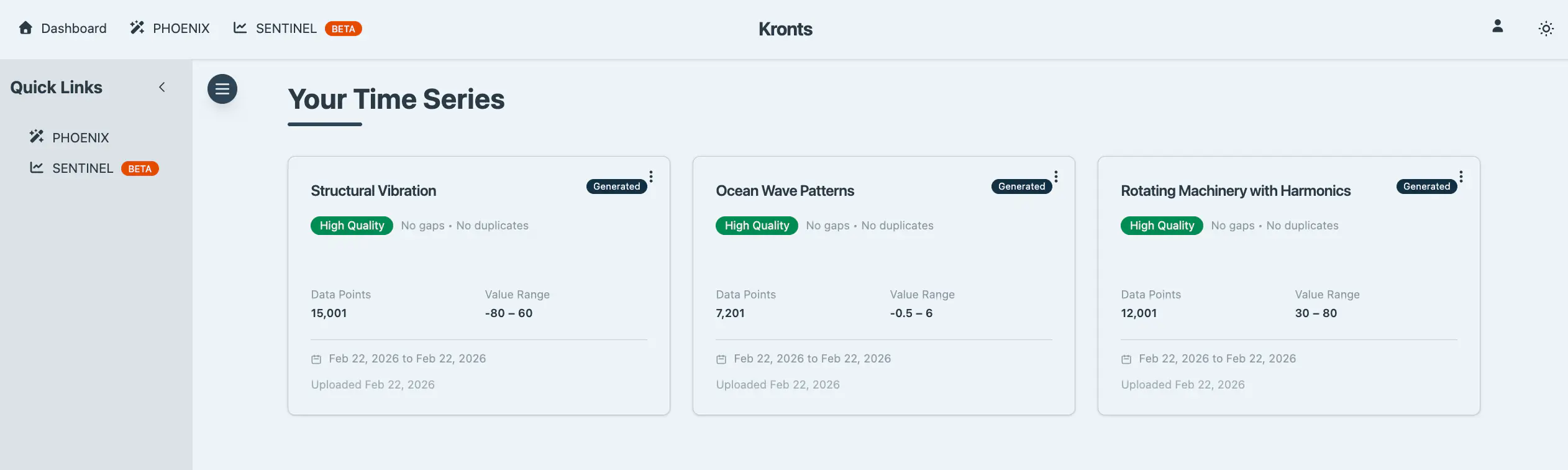
Data Persistence and Export

Once you’ve generated the perfect dataset, you have two options: save it to your personal library in the application (up to 3 datasets with 10,000 points each on the free tier) or download it directly to your local machine. Saved datasets appear in your dashboard for quick access whenever you need them.

Save to Database

Store generated datasets with custom names and descriptions for easy retrieval and organization. For efficiency, datasets with 10,000 points or fewer are stored as JSON, fast and lightweight. For larger datasets, I have TimescaleDB hypertables ready on the backend to handle them with optimal performance and scalability. This feature isn't publicly available yet, but if you're interested in accessing it, reach out.

Direct Download

Download your generated data immediately in three standard formats:

CSV (.csv): Plain text format with timestamp and value columns for universal compatibility
Excel (.xls): XML-based spreadsheet format that opens directly in Microsoft Excel and similar applications
JSON (.json): Structured format including generation metadata, statistics, and timestamped data points

All downloads are processed client-side in the browser, providing instant export without server round-trips. Files are automatically named with ISO timestamps for easy organization.

Why This Matters

Building data science workflows shouldn’t be blocked by the lack of realistic test data. Before PHOENIX, I’d spend hours writing one-off scripts to generate synthetic data for validation, only to abandon them once the project was done. Now, instead of reinventing the wheel thousands of times, you have a reusable tool that lets you iterate quickly on your algorithms without waiting for production datasets or dealing with data access constraints. Whether you’re prototyping a new outlier detection model, validating a time series forecasting pipeline, or training a team on data quality issues, PHOENIX lets you focus on the problem at hand—not on data preparation logistics. It’s the difference between spending a week engineering test data and spending five minutes generating exactly what you need.

How Much Data can I Generate?

At the moment it is possible to save up to 3 different time series with a maximum of 10,000 data points each. We’ll see how this evolves. If there is demand can increase the limits or setup a pay-to-generate system. But for the time being, this is it.

NOTE: Download as many synthetic time series as you want. The limit is only to save and persist them to the database.

PHOENIX: Simple and Efficient Synthetic Time Series Generator App