Simulating Real-World Shocks: How to Generate Transient Events in Synthetic Time Series

A seismometer records an earthquake. An accelerometer captures a hammer strike. A pressure sensor logs a valve slamming shut. A buoy records a tsunami.

These moments, sudden, violent, crucial, are transient events. They’re what engineers study, what detection algorithms need to understand, and what separates routine operation from critical failure or destructive events.

Time series with steady state signals, oscillations, noise, gentle trends are great. But these don’t simulate a realistic shock with proper ringing and decay.

🐦‍🔥 PHOENIX changes that.

What Makes a Transient Different?

Oscillations repeat. A 30 Hz sine wave cycles forever across your signal, perfect for rotating machinery or AC power lines.

Transients are localized in time. They spike suddenly, peak sharp, then fade back to zero. For example, the sound from a guitar string: vibration starts at one moment, rings at the string’s natural frequency, gradually dies. That’s a transient.

Mathematically, 🐦‍🔥 PHOENIX models them as second-order system responses, the same equations that describe how buildings sway in earthquakes, how shock absorbers cushion impacts, how electrical circuits respond to switched loads.

The physics is real. The parameters are simple. You get authentic behavior without implementing the math in code.

Five Parameters. Infinite Scenarios

Every transient in 🐦‍🔥 PHOENIX is controlled by five parameters:

1. Onset Time (s): Seconds from the start when the event happens.
2. Amplitude: Peak magnitude of the vent. This parameters inherits the unit of the event being simulated by the time series (e.g. acceleration in m/s2).
3. Natural Frequency (Hz): Oscillation frequency of the system. This determines the oscillation spacing in the event.
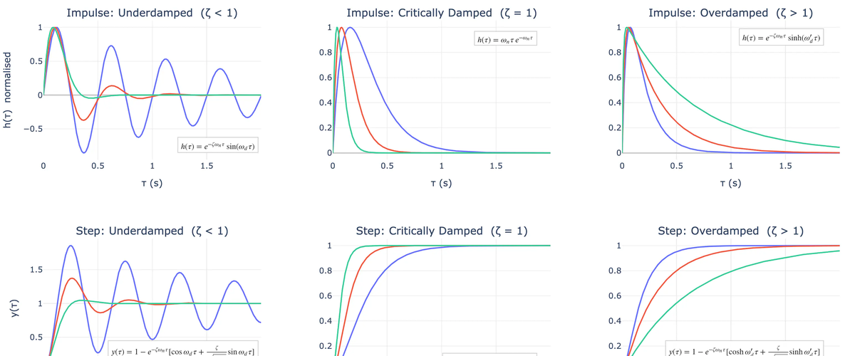
4. Damping Ratio (ζ): The damping ratio controls how quickly a system returns to rest after a disturbance. Choosing the right value depends on the physical behavior you want to replicate.
5. Response Type: Impulse (a hit) or Step (a sustained change)

That’s it. Five parameters to simulate almost any transient scenario on Earth.

Before looking at what canonical transient events look like, it is important to understand the Damping Ratio (ζ) and how it determines the magnitude and shape of the event.

ζ = 0.02 — Lightly damped, prolonged ringing

Use this for structures or systems with very little energy dissipation, such as steel frames, lightly welded joints, or metallic resonators. The signal will oscillate for many cycles before decaying. If your recorded data shows the response “ringing” for a long time after impact, this is the appropriate range.

ζ = 0.10 — Moderate ringing, gradual decay

A good starting point for geotechnical or civil applications, such as natural soil response or concrete structures. The oscillation is noticeable but fades within a reasonable number of cycles. Use this when the system has some inherent energy dissipation but is not tightly controlled.

ζ = 0.50 — Brief overshoot, rapid decay

Suitable for instrumentation and measurement systems where you expect a single overshoot followed by quick settling. Typical of sensor housings, spring-mounted instruments, or lightly cushioned mechanical assemblies. The response looks like a single bounce before stabilizing.

ζ = 1.00 — Critically damped, no oscillation

The system returns to equilibrium as fast as physically possible without any overshoot. Use this for precision sensors, control actuators, or any application where oscillation is undesirable and fastest settling time matters. There is no ringing — the signal decays smoothly and directly.

ζ > 1.00 — Overdamped, slow sluggish return

The system is over-constrained and returns to rest more slowly than critical damping, with no oscillation whatsoever. Use this for heavily damped mechanical systems such as hydraulic dashpots, thick rubber mounts, or viscous isolation systems. The response looks like a slow exponential decay.

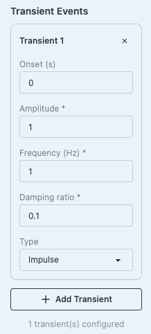
To visualize how these parameters work together, the figure below shows the complete landscape of second-order system responses across the full range of damping ratios. The top row displays impulse responses, the signature of a sudden impact or hit, where you can see how the damping ratio fundamentally reshapes the character of the transient. Underdamped systems (ζ < 1) exhibit multiple oscillations that gradually decay, mimicking the ringing you'd observe from striking a bell or dropping an object on a suspended platform. Critically damped systems (ζ = 1) settle with a smooth, direct approach to zero without any overshoot, the fastest possible return to rest without oscillation. Overdamped systems (ζ > 1) decay even more slowly, showing the sluggish, non-oscillatory behavior characteristic of heavily constrained mechanisms. The bottom row shows step responses, the signature of a sudden sustained change, where you see the system's approach to a new equilibrium rather than return to zero. Notice how higher natural frequencies (fn) compress the time scale of the response, allowing you to simulate fast or slow systems simply by adjusting this single parameter. By varying these five parameters, you're essentially controlling the physics of your synthetic event: how it starts, how it oscillates or doesn't oscillate, and how quickly it settles back down.

Example: Simulated Seismograph Time Series

Let’s make something concrete, a vertical-component seismograph recording of a local earthquake. A seismograph time series will require:

1. Background hum: ambient ground vibration
2. P-wave arrival: fast, sharp, moderate energy
3. S-wave arrival: slower, bigger, lower frequency

Here’s how to set it up in 🐦‍🔥 PHOENIX:

Base Signal:

• Mean: 0 mm/s (velocity centered on quiet)
• Noise: 0.5 mm/s (ambient microseisms)

P-wave (Transient 1):

• Onset: 5 seconds
• Amplitude: 50 mm/s
• Frequency: 8 Hz (typical compression)
• Damping: 0.06
• Type: Impulse

S-wave (Transient 2):

• Onset: 15 seconds
• Amplitude: 120 mm/s (carries more energy)
• Frequency: 3 Hz (lower shear wave)
• Damping: 0.04
• Type: Impulse

Time Config:

• Duration: 60 seconds
• Sample rate: 100 Hz

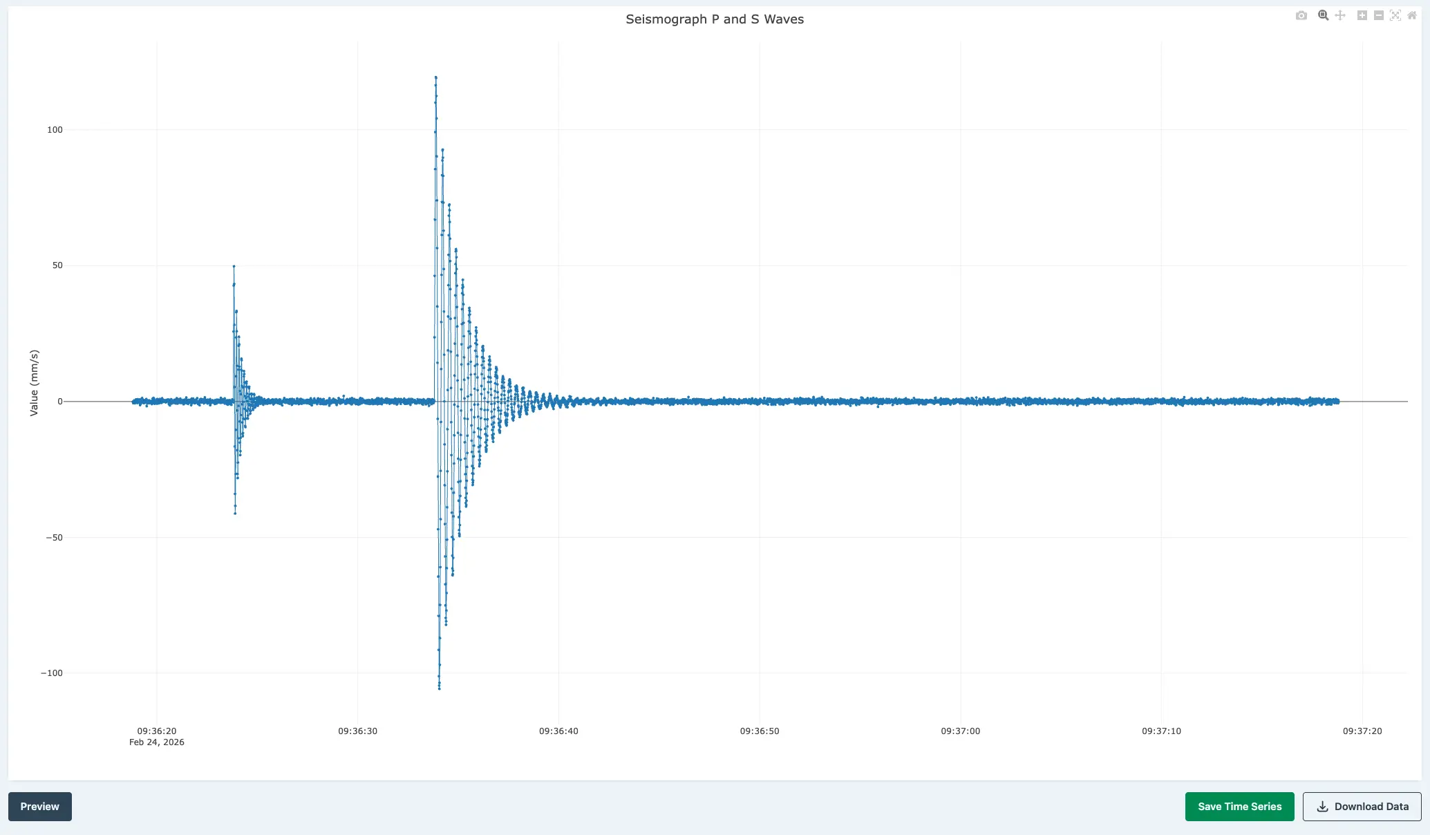
The output looks unmistakably like a seismograph: quiet noise floor, sharp P-wave spike with high-frequency ringing, then a larger S-wave with deeper frequencies. No guessing. No tweaking. Just physics.

You Don’t Need to Know the Math

🐦‍🔥 PHOENIX’s AI agent saves you hours:

“Simulate a 60-second vertical seismograph recording with a P-wave at 5 seconds and S-wave at 15 seconds. Use realistic frequencies and damping for a local earthquake about 50 km away.”

Or give it an image and describe what you want, as shown in this video.

The agent knows:

• P-waves are higher frequency than S-waves
• S-waves pack more amplitude
• Seismic damping ratios live in the 0.02–0.10 range
• Local vs. distant earthquakes look different

It translates English into the right parameters and generates the signal. No parameter hunting. No domain expertise required.

Beyond Earthquakes

The same model applies everywhere:

Impact Testing
Engineers strike structures to measure natural frequencies. Generate this with high frequency (10–100 Hz), very low damping (0.01–0.03), impulse response.

Water Hammer
Valve closure sends pressure waves bouncing through pipes. Model with step response, low frequency (1–5 Hz), moderate damping (0.10–0.20).

Electrical Switching
Circuit breaker operations create transient oscillations. Use high frequency (50–500 Hz), moderate-to-high damping, impulse response.

Thermal Shock
Sudden temperature swings in industrial processes. Very low frequency (0.01–0.1 Hz, because heat moves slowly), overdamped (ζ > 1, temperature doesn’t oscillate), step response.

The same five parameters handle all of it.

The Damping Shortcut

Choosing damping ratio is the hardest part. Here’s the trick: if you know how long you want decay to take, calculate it:

ζ = 4 / (t_decay × 2π × fₙ)

Example 1: You want a 45 Hz impact to ring out in 2 seconds.

ζ = 4 / (2 × 6.283 × 45) = 0.007

Very light damping—makes sense for ~90 oscillation cycles.

Example 2: You want a 3 Hz seismic wave to fade in 10 seconds.

ζ = 4 / (10 × 6.283 × 3) = 0.021

Light damping again—consistent with how seismic energy actually decays.

Plug in your decay time and natural frequency, solve for ζ, done.

Combining Everything

Real sensor data never has transients alone. They sit on top of:

• Continuous oscillations (machinery, waves)
• Trends (drift, aging)
• Noise (always present)
• Multiple channels (correlated)

Phoenix stacks them additively:

signal = mean + trend + oscillations + transients + noise

Create machine vibration with an impact at t=5s. Layer a temperature drift with a thermal shock. Build a three-channel seismograph with different amplitudes per component.

Everything combines naturally.

Quick Practical Tips

Start with impulse. It’s more common and easier to visualize. Graduate to step only for sustained changes.

Keep noise low relative to the transient. Aim for 10:1 signal-to-noise or better. For testing detection algorithms, lower it to create harder scenarios.

Space out multiple transients. Let each one decay before the next begins. Estimate decay time as 4 / (ζ × 2π × fₙ) seconds.

Match your sampling rate to frequency. Use at least 2.5× the natural frequency. A 45 Hz transient needs ≥112.5 Hz sampling.

What This Means for You

Transient events are the latest addition to Phoenix’s toolkit. Combined with oscillations, trends, noise, multichannel correlations, and data degradation, they let you simulate virtually any industrial time series.

The breakthrough: you describe the physical scenario in plain English. The AI handles the math.

No parameter tables. No signal processing textbooks. No reverse-engineering from real data.

Just: What does your sensor capture in the real world? Describe it. Phoenix generates it.

Try it: Open Phoenix. Describe a shock event in your domain—a valve slam, a structural impact, a seismic arrival, whatever matters to you. See how realistic the output looks.

You might be surprised how close synthetic data can get to the real thing.